All you need to know about investing short and simple
© Leonardo Timis
CHAPTER 8
THE BEST STRATEGIES - empirical research
8.1 Introduction
In summary, this chapter will present for each investment strategy exposed in chapter 6: histogram distribution, range, arithmetic mean, median, assets under management weighted mean, assets under management weighted standard deviation, and assets under management weighted coefficient of variation of the monthly risk-adjusted performance (Sharpe ratio) observed over the last ten years.
A strategy performance is here defined as the mean of the Sharpe ratios of all those hedge funds present in our sample that systematically applied that strategy, weighted by assets under management. The reason for this choice of weighting the mean lies in the fact that a smaller fund cannot have the same weight as a bigger fund in the representation of its investment class.
Successively, the performance of each strategy will be compared to two fundamental benchmarks, respectively the S&P 500 index and the MSCI AWCI index; the first one is a national index while the second one is a global index.
Finally, we will perform hypothesis tests on the previous comparations to understand if the discrepancy of a strategy performance over an index performance was statistically significant.
8.2 Empirical data
The empirical analysis that follows is based on data gathered from the Morningstar database. The initially extracted excel data from Morningstar included monthly returns from July 2009 to May 2019 of all the hedge funds still available on the database, for a total of 3364 hedge funds.
Successively, using VBA, I polished the initially extracted excel data to obtain an actual sample to work on, keeping only the hedge funds expressed in US dollars because those expressed in Euro were too few for an extensive analysis from which is possible to obtain significant conclusions. Furthermore, I rejected those hedge funds that presented lacks in their monthly returns, I rejected those hedge funds that did not specify the size of their fund in terms of assets under management because necessary for the weighting, and I rejected those hedge funds the presented mixed investment strategies.
In the end, from an initial base of 3364 hedge funds, I remained with 402 hedge funds.
Finally, I reordered the remaining hedge funds by investment strategy. For each hedge fund, I calculated the average monthly return, the standard deviation of the monthly returns, and the monthly Sharpe ratio - as the average monthly return of the risk-free security denominated in US dollars was known as well.
Now that we have the monthly Sharpe ratios of each hedge fund and we have divided them by strategy class, we can start presenting the empirical analysis.
8.3 Strategies analysis
With regards to the long/short equity strategy, the number of hedge funds included in this class is 177 representing by far the most adopted strategy, of which 7 Asia/pacific long/short equity, 11 Europe long/short equity, 25 global long/short equity, 14 long-only equity, 92 US long/short equity, 28 US small cap long/short equity.
The histogram distribution of the Sharpe ratios of this strategy is the following.
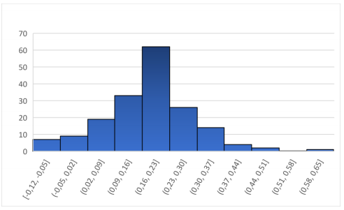
Considering that the maximum value observed is 0.59 while the minimum value observed is -0.12, the range is 0.71, the arithmetic mean is 0.18 and the median is 0.18.
Since in excel there are not functions to calculate a weighted mean and a weighted standard deviation, these values were calculated manually dividing the sum of the products of the Sharpe ratios and the distances from the mean by the sum of the weights, which is the sum of the assets under management.
Following the just described reasoning, the assets under management weighted mean of the Sharpe ratios is 0.23, greater than 0.18, while the assets under management weighted standard deviation of the Sharpe ratios is 0.10.
Finally, the assets under management weighted coefficient of variation is equal to the ratio of the two values we have just found, in this case 0.45.
With regards to the dedicated short or short selling strategy, there are no hedge funds appearing in our sample, confirming the already made affirmation that states that this very risky strategy is not much applied.
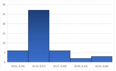
With regards to the global macro strategy instead, in our sample there are 35 hedge funds that follow this strategy.
The histogram distribution of the Sharpe ratios of this strategy is the following.

Considering that the maximum value observed is 0.29 while the minimum value observed is -0.08, the range is 0.37, the arithmetic mean is 0.09 and the median is 0.09.
Once again, since in excel there are not functions to calculate a weighted mean and a weighted standard deviation, these values were calculated manually dividing the sum of the products of the Sharpe ratios and the distances from the mean by the sum of the weights, which is the sum of the assets under management.
Following the just described reasoning, the assets under management weighted mean of the Sharpe ratios is 0.21, decisively greater than 0.09, while the assets under management weighted standard deviation of the Sharpe ratios is 0.13.
Finally, the assets under management weighted coefficient of variation is equal to the ratio of the two values we have just found, in this case 0.59.
With regards to the emerging markets strategy, in our sample there are 41 hedge funds that follow this strategy, of which 33 emerging markets long/short equity and 8 emerging markets long-only equity.
The histogram distribution of the Sharpe ratios of this strategy is the following.

Considering that the maximum value observed is 0.45 while the minimum value observed is 0.01, the range is 0.44, the arithmetic mean is 0.14 and the median is 0.13.
Once again, since in excel there are not functions to calculate a weighted mean and a weighted standard deviation, these values were calculated manually dividing the sum of the products of the Sharpe ratios and the distances from the mean by the sum of the weights, which is the sum of the assets under management.
Following the just described reasoning, the assets under management weighted mean of the Sharpe ratios is 0.18, greater than 0.14, while the assets under management weighted standard deviation of the Sharpe ratios is 0.08.
Finally, the assets under management weighted coefficient of variation is equal to the ratio of the two values we have just found, in this case 0.42.
With regards to the managed futures strategy, in our sample there are 61 hedge funds that follow this strategy.
The histogram distribution of the Sharpe ratios of this strategy is the following.

Considering that the maximum value observed is 0.27 while the minimum value observed is -0.11, the range is 0.38, the arithmetic mean is 0.07 and the median is 0.06.
Once again, since in excel there are not functions to calculate a weighted mean and a weighted standard deviation, these values were calculated manually dividing the sum of the products of the Sharpe ratios and the distances from the mean by the sum of the weights, which is the sum of the assets under management.
Following the just described reasoning, the assets under management weighted mean of the Sharpe ratios is 0.11, greater than 0.07, while the assets under management weighted standard deviation of the Sharpe ratios is 0.07.
Finally, the assets under management weighted coefficient of variation is equal to the ratio of the two values we have just found, in this case 0.60.
With regards to the equity market neutral strategy, in our sample there are 8 hedge funds that follow this strategy.
The histogram distribution of the Sharpe ratios of this strategy is the following.

Considering that the maximum value observed is 0.67 while the minimum value observed is 0.07, the range is 0.60, the arithmetic mean is 0.23 and the median is 0.20.
Once again, since in excel there are not functions to calculate a weighted mean and a weighted standard deviation, these values were calculated manually dividing the sum of the products of the Sharpe ratios and the distances from the mean by the sum of the weights, which is the sum of the assets under management.
Following the just described reasoning, the assets under management weighted mean of the Sharpe ratios is 0.23, equal to the arithmetic mean, while the assets under management weighted standard deviation of the Sharpe ratios is 0.03.
Finally, the assets under management weighted coefficient of variation is equal to the ratio of the two values we have just found, in this case 0.15.
With regards to the fixed income arbitrage strategy, in our sample there are 16 hedge funds that follow this strategy.
The histogram distribution of the Sharpe ratios of this strategy is the following.

Considering that the maximum value observed is 0.52 while the minimum value observed is -0.12, the range is 0.65, the arithmetic mean is 0.35 and the median is 0.37.
One more time, since in excel there are not functions to calculate a weighted mean and a weighted standard deviation, these values were calculated manually dividing the sum of the products of the Sharpe ratios and the distances from the mean by the sum of the weights, which is the sum of the assets under management.
Following the just described reasoning, the assets under management weighted mean of the Sharpe ratios is 0.40, greater than 0.35, while the assets under management weighted standard deviation of the Sharpe ratios is 0.07.
Finally, the assets under management weighted coefficient of variation is equal to the ratio of the two values we have just found, in this case 0.18.
With regards to the convertible arbitrage strategy, in our sample there are 4 hedge funds that follow this strategy.
The histogram distribution of the Sharpe ratios of this strategy is the following.

Considering that the maximum value observed is 0.48 while the minimum value observed is 0.24, the range is 0.24, the arithmetic mean is 0.35 and the median is 0.34.
One more time, since in excel there are not functions to calculate a weighted mean and a weighted standard deviation, these values were calculated manually dividing the sum of the products of the Sharpe ratios and the distances from the mean by the sum of the weights, which is the sum of the assets under management.
Following the just described reasoning, the assets under management weighted mean of the Sharpe ratios is 0.45, greater than 0.35, while the assets under management weighted standard deviation of the Sharpe ratios is 0.12.
Finally, the assets under management weighted coefficient of variation is equal to the ratio of the two values we have just found, in this case 0.26.
With regards to the event driven strategy, in our sample there are 44 hedge funds that follow this strategy, of which 12 merger arbitrage and 32 other types of event driven strategies.
The histogram distribution of the Sharpe ratios of this strategy is the following.
Considering that the maximum value observed is 0.61 while the minimum value observed is 0.01, the range is 0.60, the arithmetic mean is 0.25 and the median is 0.22.
One more time, since in excel there are not functions to calculate a weighted mean and a weighted standard deviation, these values were calculated manually dividing the sum of the products of the Sharpe ratios and the distances from the mean by the sum of the weights, which is the sum of the assets under management.
Following the just described reasoning, the assets under management weighted mean of the Sharpe ratios is 0.29, greater than 0.25, while the assets under management weighted standard deviation of the Sharpe ratios is 0.09.
Finally, the assets under management weighted coefficient of variation is equal to the ratio of the two values we have just found, in this case 0.31.
With regards to the distressed securities strategy, in our sample there are 15 hedge funds that follow this strategy.
The histogram distribution of the Sharpe ratios of this strategy is the following.

Considering that the maximum value observed is 0.76 while the minimum value observed is 0.05, the range is 0.70, the arithmetic mean is 0.36 and the median is 0.32.
One more and for the last time, since in excel there are not functions to calculate a weighted mean and a weighted standard deviation, these values were calculated manually dividing the sum of the products of the Sharpe ratios and the distances from the mean by the sum of the weights, which is the sum of the assets under management.
Following the just described reasoning, the assets under management weighted mean of the Sharpe ratios is 0.50, far greater than 0.36, while the assets under management weighted standard deviation of the Sharpe ratios is 0.21.
Finally, the assets under management weighted coefficient of variation is equal to the ratio of the two values we have just found, in this case 0.43.
8.4 Benchmarks comparison
The analysis of the previous strategies is summarized in the following table, where we also added the performances of the S&P 500 and the MSCI ACWI over the same period, which starts from July 2009 to May 2019.

We observe that the only strategies that beat the S&P 500 over this period were: fixed income arbitrage, convertible arbitrage, and distressed securities.
While the strategies that beat the MSCI ACWI over this period were: long/short equity, global macro, equity market neutral, fixed income arbitrage, convertible arbitrage, event driven, and distressed securities.
But, are these performance superiorities only a case, or are they statistically significant?
8.5 Hypotheses testing


8.6 Conclusions
After we analyzed the risk-adjusted performances of the strategies over the last circa ten years, we observed that some strategies beat the S&P 500 and MSCI ACWI indexes; thus, we subjected these results to the hypotheses testing to understand if these performance superiorities were robust from a statistical point of view, given a significance level of 5%.
From our testing, we discovered that the strategies that beat the S&P 500 in a statistically significant way are: fixed income arbitrage, convertible arbitrage, and distressed securities.
While the strategies that beat the MSCI ACWI in a statistically significant way are: long/short equity, equity market neutral, fixed income arbitrage, convertible arbitrage, event driven, and distressed securities.
Only comparing global macro to MSCI ACWI, we found that it does not subsist enough empirical evidence to affirm its superiority.
Bibliography and sitography
of the second part of this book
Bodie, Z. et al. (2018). Investments. 11. Ed. New York: McGraw-Hill Education.
Fabrizi, P.L. et al. (2016). Economia del mercato mobiliare. 6. Ed. Milano: EGEA S.p.A.
Ferrari, P. et al. (2019). Asset management e investitori istituzionali. 2. ed. Milano: Pearson Italia.
Lederman, J. (1995). Hedge funds. Investment portfolio strategies for the institutional investor. New York: McGraw-Hill.
Lhabitant, F.S. (2006). Handbook of hedge funds. Chichester: John Wiley & Sons, Ltd.
Newbold, P. et al. (2010). Statistica. 2. Ed. Milano: Pearson Italia.
Philips, K.S. et al. (2003). Hedge funds. Definitive strategies and Techniques. Hoboken: Wiley.
Smith, D.M. (2017) Hedge funds: structure, strategies, and performance. New York: Oxford University Press.
Zask, E. (2013). All about hedge funds. 2. Ed. New York: McGraw-Hill.
For those, like me, that like keeping the physical copy of a book on their bookshelves, you can buy the original copy of this book on Amazon store for $34.
For those more addicted to Kindle, you can buy a copy of this book on Kindle store for $24.